Python client library

Overview

This is documentation for the Python library of Sweat Stack. This library provides a seamless interface to interact with the Sweat Stack API, allowing users to retrieve, analyze, and visualize activity data and performance metrics.

Installation

We recommend using uv to manage Python and install the library. Read more about uv here.

uv pip install sweatstack

You can also install it with pip (or pipx) directly.

python -m pip install sweatstack

Quickstart

Sweatlab

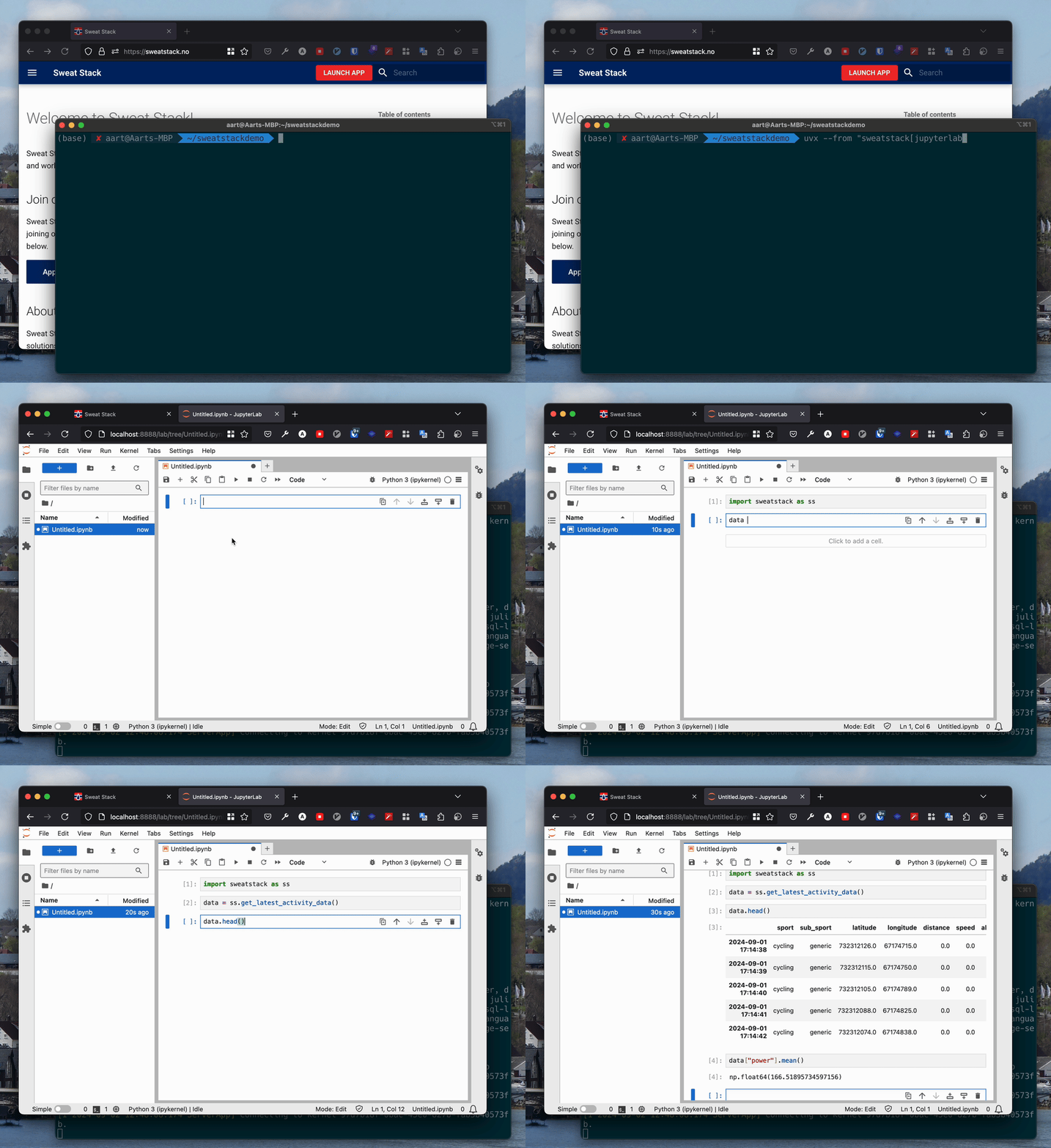
If you have uv installed, the fastest way to get started is to run the following command in your terminal:

uvx --from "sweatstack[jupyterlab]" sweatlab

This will open a JupyterLab instance with the SweatStack library pre-imported and authenticated via the browser authentication flow.

Sweatshell

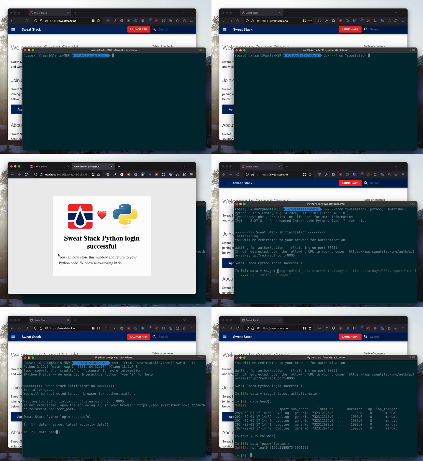
uvx --from "sweatstack[ipython]" sweatshell

This will open an interactive Python shell with the SweatStack library pre-imported and it will automatically trigger the browser authentication flow.

Other Python environments

Alternatively, you can use any Python environment of your choice, install the library (see above) and get started:

import sweatstack as ss

ss.login()

latest_activity = ss.get_latest_activity()

print(latest_activity)  # `latest_activity` is a Pydantic model

Authentication

To be able to access your data in Sweat Stack, you need to authenticate the library with your Sweat Stack account. When using Python in the browser or with the sweatlab or sweatshell command, this is done automatically. If you want to authenticate from code in another Python environment, you can use the login() method:

import sweatstack as ss

ss.login()

This will automaticallyset the appropriate authentication tokens in your Python code.

Alternatively, you can set the SWEAT_STACK_API_KEY environment variable to your API key directly. You can create an API key on your account page.

import os

import sweatstack as ss

os.environ["SWEAT_STACK_API_KEY"] = "your_api_key_here"

# Now you can use the library

Please note that hardcoding your API key into your code is not recommended if you are sharing your code with others.

Activities

To list activities, you can use the list_activities() function:

import sweatstack as ss

activities = ss.list_activities()
activities

By default, this methods returns a pandas DataFrame. If you want a list of Pydantic models, you can set the as_dataframe parameter to False:

import sweatstack as ss

for activity in ss.list_activities(as_dataframe=False):
    # Do something with the activity
    pass

The list_activities() method returns a summary of the activities, not the actual timeseries data. To get the actual data, you need to use the get_activity_data() or get_latest_activity_data()) methods documented below.

Activity details

To get the details of an activity, you can use the get_activity() function:

import sweatstack as ss

activity = ss.get_activity(activity_id)
activity

To quickly the latest activity, you can use the get_latest_activity() function:

import sweatstack as ss

activity = ss.get_latest_activity()

Activity data

To get the timeseries data of one activity, you can use the get_activity_data() method:

import sweatstack as ss

data = ss.get_activity_data(activity_id)
data

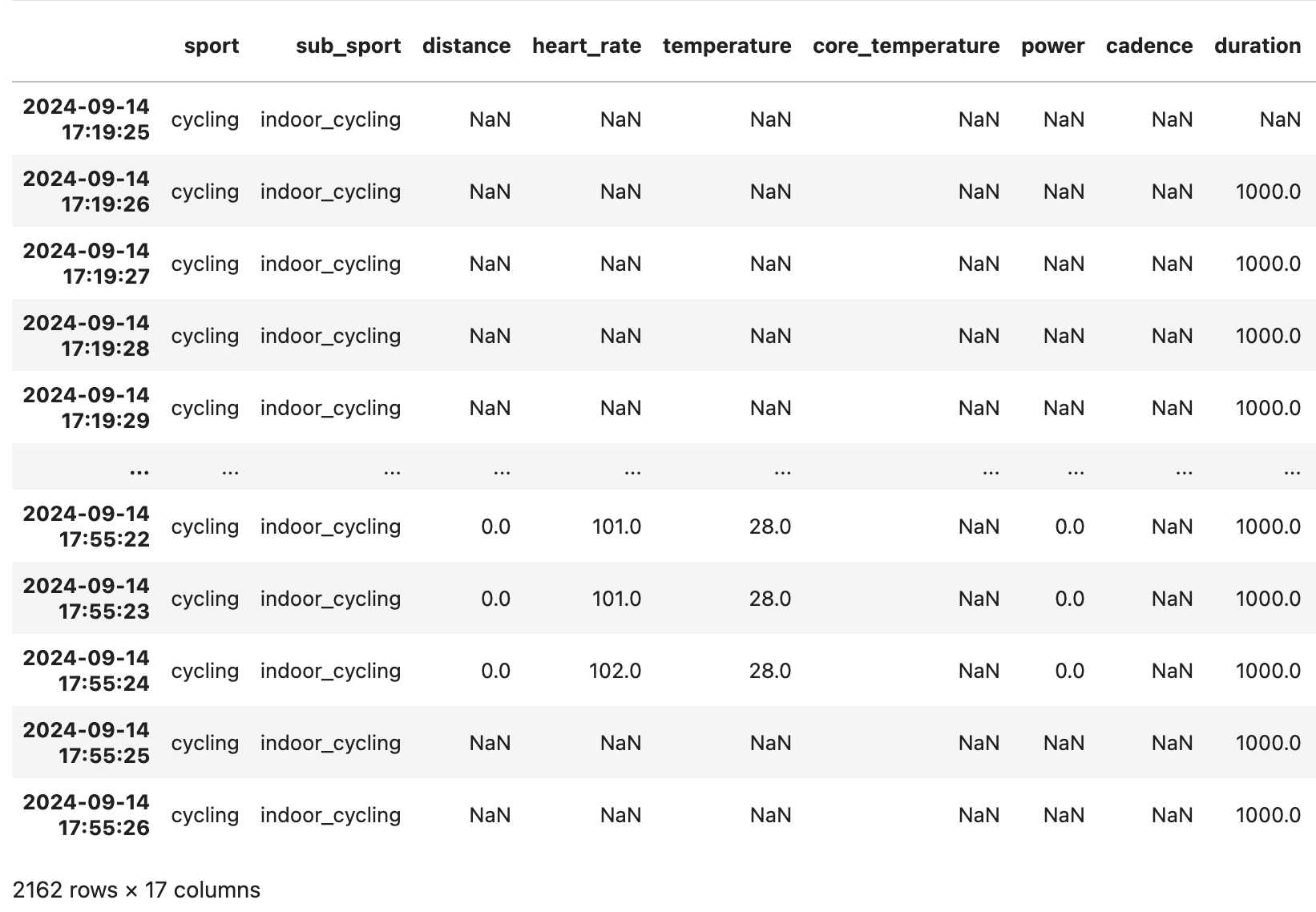
This method returns a pandas DataFrame. If your are not familiar with pandas and/or DataFrames, start by reading this introduction.

Similar as for the summaries, you can use the get_latest_activity_data() method to get the timeseries data of the latest activity:

import sweatstack as ss

data = ss.get_latest_activity_data()

Longitudinal Data

To get the timeseries data of multiple activities, you can use the get_longitudinal_data() method:

from datetime import date, timedelta

import sweatstack as ss

longitudinal_data = ss.get_longitudinal_data(
    start=date.today() - timedelta(days=180),
    sport="running",
    metrics=["power", "heart_rate"],
)

This returns a pandas DataFrame similar to the one returned by get_activity_data().

Because the result of get_longitudinal_data() can be very large, the data is retrieved in a compressed format (parquet) that requires the pyarrow library to be installed. If you intend to use this method, make sure to install the sweatstack library with this extra dependency:

uv pip install sweatstack[parquet]

Also note that depending on the amount of data that you requested, this might take a while.

Plotting

To plot data, there are a few plotting methods available.

import sweatstack as ss

ss.plot_activity_data(activity_id)

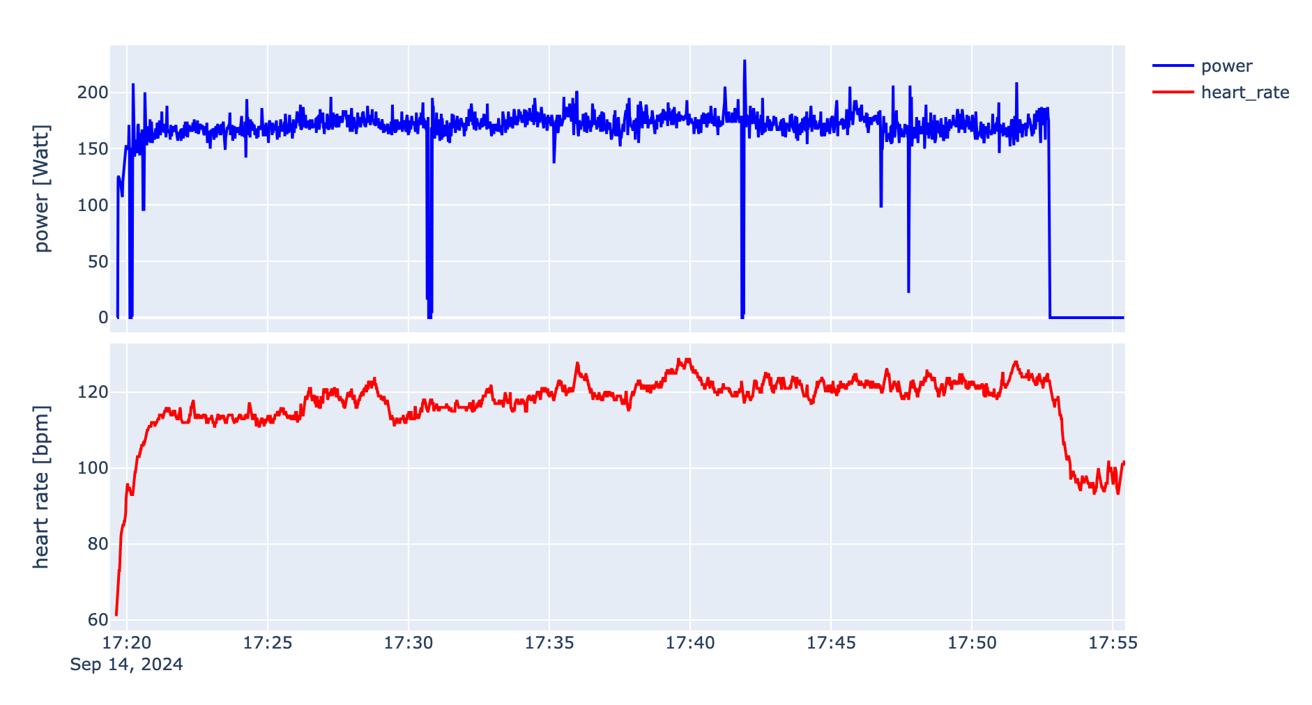
...wil plot the all the available columns from the specified activity. There is also a ss.plot_latest_activity_data() method that will plot the latest activity data.

All of these methods accept a metrics argument, which is a list of metrics that you want to plot, as well as a subplots argument, which is a boolean that specifies whether you want to plot each metrics in subplots or not. Example:

import sweatstack as ss

ss.plot_latest_activity_data(metrics=["heart_rate", "power"], subplots=True)

There is also a ss.plot_scatter() method that you can use to plot a scatter plot of any two metrics:

import sweatstack as ss

ss.plot_scatter(x=data["power"], y=data["heart_rate"])

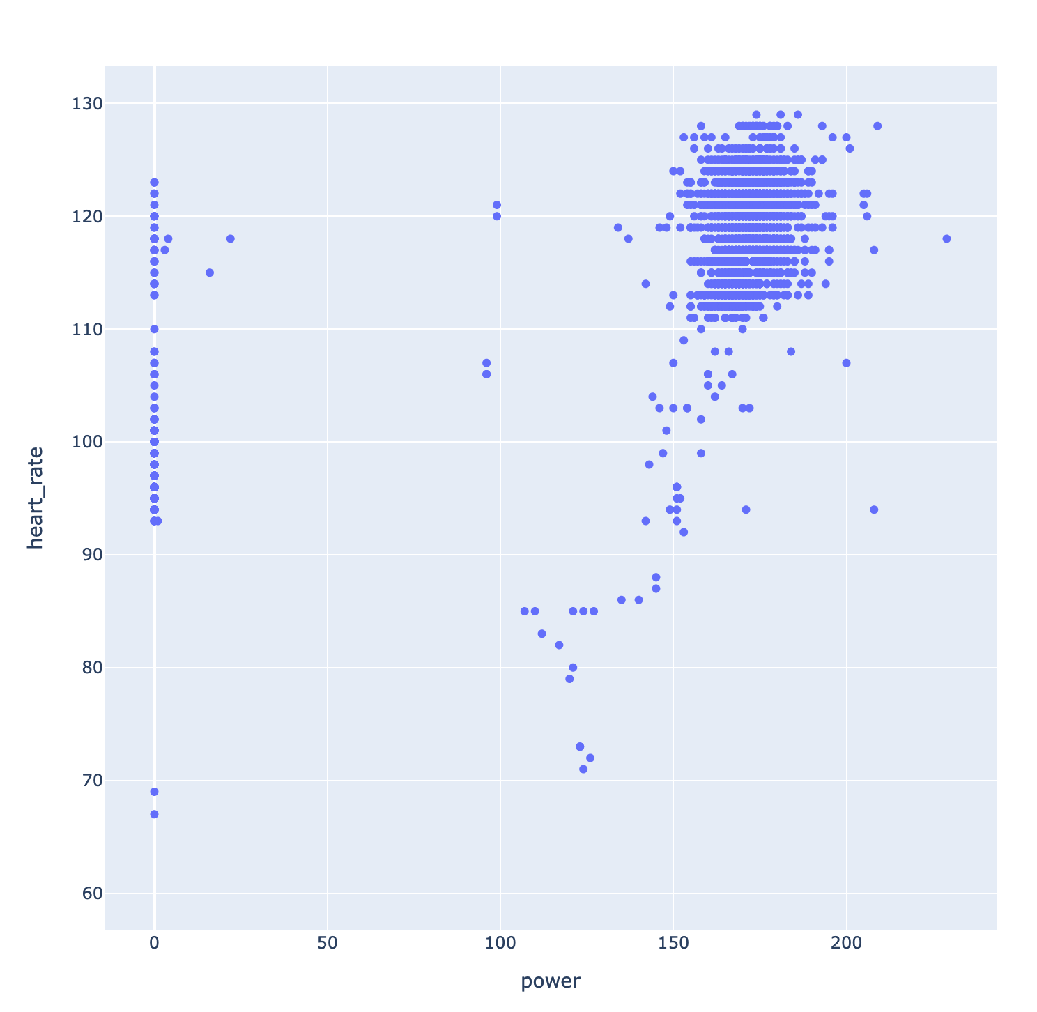
For plotting mean-max data, you can use the ss.plot_mean_max() method:

import sweatstack as ss

ss.plot_mean_max(
    sport="running",
    metric="power",
)

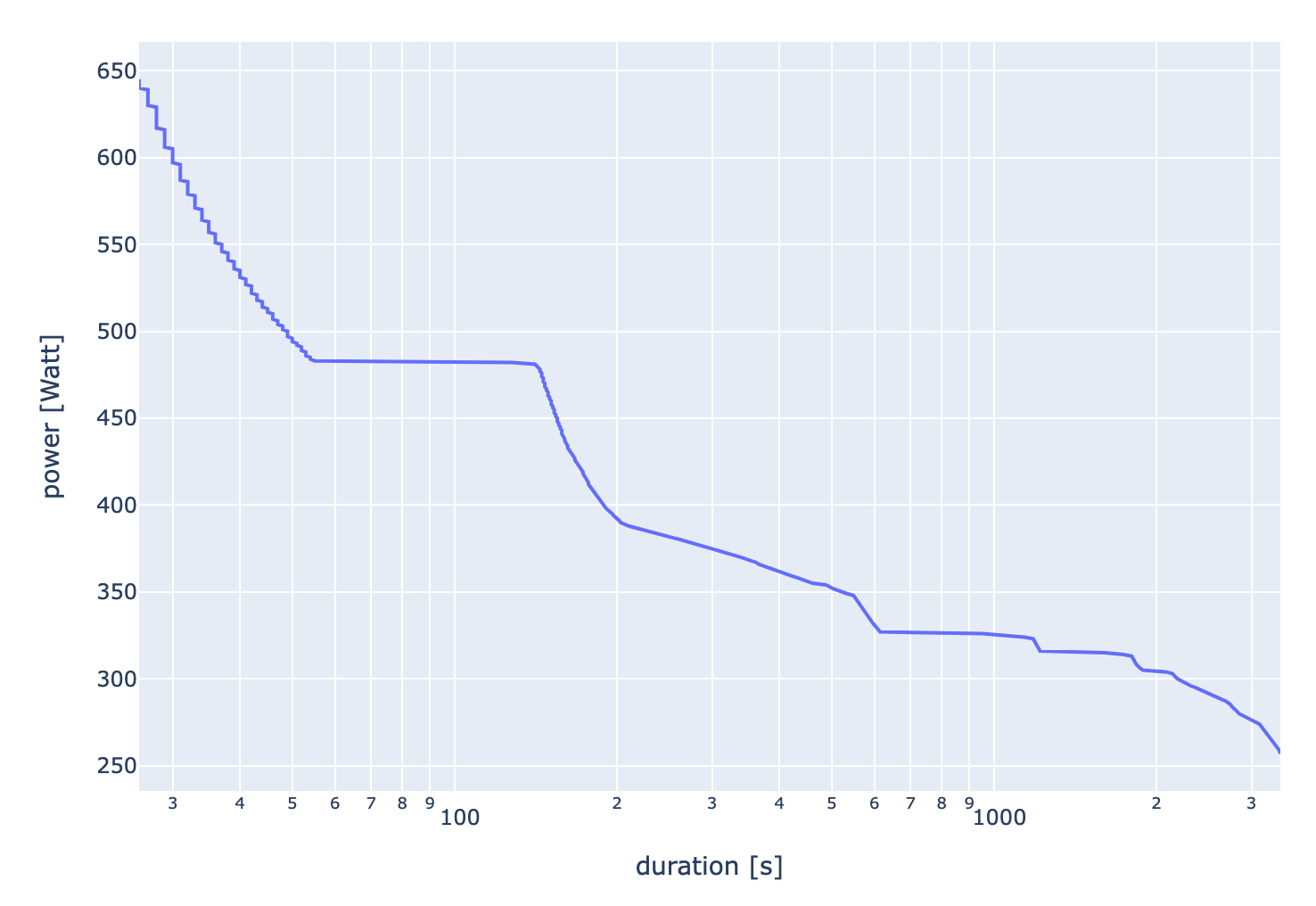
By default, this method will plot the mean-max data for the last 30 days. But you can provide explicit start and end dates (both optional) to plot the mean-max data for a different time period and these can provided as both date objects and str objects (e.g. "1970-01-01").

from datetime import date, timedelta

import sweatstack as ss

ss.plot_mean_max(
    sport="running",
    metric="power",
    start=date.today() - timedelta(days=180),
    end=date.today(),
)

To plot the mean-max data for multiple time windows, you can provide a list of start and end dates as the windows argument:

from datetime import date, timedelta

import sweatstack as ss

ss.plot_mean_max(
    sport="running",
    metric="power",
    windows=[
        (date.today() - timedelta(days=30), date.today()),
        (date.today() - timedelta(days=60), date.today() - timedelta(days=30)),
    ],
)

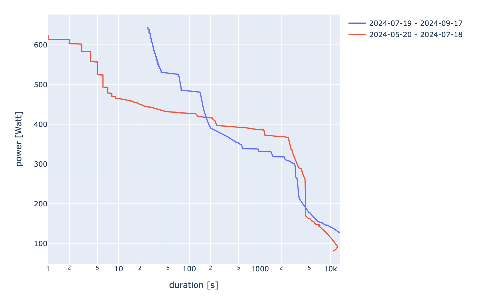
This opens up a lot of possibilities, for example to plot the mean-max data for each 30 day window in the last 300 days:

from datetime import date, timedelta

import sweatstack as ss

ss.plot_mean_max(
    sport="running",
    metric="power",
    windows=[(date.today() - timedelta(days=i + 30), date.today() - timedelta(days=i + 1)) for i in range(0, 120, 30)],
)

At the moment, only the Plotly plotting backend is available, but more plotting backends (like Matplotlib) will be added in the future.

Please note that these plotting methods are just there for your convenience. If you want to customize your plots, we recommend using a plotting library like Plotly or Matplotlib directly. This page from the pandas documentation gives a good overview of the available plotting options for the pandas.DataFrames and pandas.Series that this library returns.

Uploading

To upload activities (only .fit files at this moment), you can use the upload_activity() method:

ss.upload_activity("path/to/activity.fit")

To upload multiple activities, you can use the batch_upload_activities() method:

ss.batch_upload_activities(files=["path/to/activity1.fit", "path/to/activity2.fit", "path/to/activity3.fit"])

For both the upload_activity() and batch_upload_activities() methods, you can pass files as a file path (string or pathlib.Path) or file-like object.

In addition to this, batch_upload_activities() also accepts a directory argument (string or pathlib.Path), allowing you to upload all activities in a directory:

ss.batch_upload_activities(directory="path/to/directory")

Metrics

The API supports the following metrics:

• power: Power in Watt
• speed: Speed in m/s
• heart_rate: Heart rate in BPM
• smo2: Muscle oxygen saturation in %
• core_temperature: Core body temperature in °C
• altitude: Altitude in meters
• cadence: Cadence in RPM
• temperature: Ambient temperature in °C
• distance: Distance in m
• longitude: Longitude in degrees
• latitude: Latitude in degrees

Sports

The API supports the following sports:

• running: Running
• cycling: Cycling

More sports will be added in the near future.